Correction schemes for electrostatic finite-size effects¶

Contents

Theoretical introduction
Implementation in Spinney
- The scheme of Freysoldt, Neugebauer and Van de Walle
- The scheme of Kumagai and Oba

Theoretical introduction ¶

The main artifact of the supercell approach for point-defect calculations consists in the introduction of periodic images of the defect located in the simulation cell. Such periodically-repeated array of defects corresponds to very high defect concentrations for commonly used supercell types.

In such case, defect-defect interactions are large and can considerably affect the predicted energy of the point defect.

Among the kinds of defect-defect interactions, electrostatic ones are never negligible for any practical supercell size.

The study of point defects in the dilute limit then requires some scheme to correct for such spurious electrostatic interactions.

The introduction of a point defect will induce a redistribution of the host material electronic charge density. In the ideal case of an isolated point defect, we call this defect-induced charge density \(\rho_{iso}\). On the other hand, in the supercell method, due to the application of periodic boundary conditions, the defect-induced charge density will be different: \(\rho_{per}\). Moreover, for charged point defects, periodic boundary conditions require the introduction of a neutralizing background, usually taken as an homogeneous jellium of density \(-\frac{q}{V}\), where \(q\) is the defect charge state and \(V\) is the supercell volume.

The defect-induced electrostatic potential can be obtained from the induced charge density by solving Poisson equation with the proper boundary conditions. This will yield the potentials \(\phi_{iso}\) and \(\phi_{per}\) for the \(\rho_{iso}\) and \(\rho_{per}\), respectively:

\[\nabla^2 \phi(\mathbf{r}) = -4\pi \rho(\mathbf{r})\]

Correction schemes for electrostatic finite-size effects assume that the point defect induces a charge density localized in the supercell. In this case the charge densities induced by periodic and isolated defect can be considered to be the same within the supercell: \(\rho_{iso} = \rho_{per} = \rho\) in \(V\). In addition:

\[q = \int_V \rho_{iso}(\mathbf{r}) \, d\mathbf{r} = \int_V \rho_{per}(\mathbf{r}) \, d\mathbf{r}\]

Considering the defect-induced electrostatic energy per supercell, what it is obtained employing periodic boundary conditions is the quantity:

\[E_{per} = \frac{1}{2} \int_V \phi_{per}(\mathbf{r}) \left( \rho(\mathbf{r}) - \frac{q}{V} \right) \, d\mathbf{r}\]

while ideally we would like to obtain:

\[E_{iso} = \frac{1}{2} \int_V \phi_{iso}(\mathbf{r}) \rho(\mathbf{r}) \, d\mathbf{r}\]

Correction schemes for electrostatic finite-size effects aim to calculate the corrective term:

(3)¶\[E_{corr} = E_{iso} - E_{per}\]

Spinney implements two state-of-the-art correction schemes:

The scheme proposed by Freysoldt, Neugebauer and Van de Walle [FNVdW09].
The scheme proposed by Kumagai and Oba [KO14].

The latter is an improvement over the former. In both cases, the correction energy of equation (3) is expressed as:

\[E_{corr} = -E_{lat} + q \Delta \phi\]

\(E_{lat}\) takes into account the interaction of \(\rho\) with the host material and the jellium background in periodic boundary conditions, while \(\Delta \phi\) is an alignment term.

\(\rho\) is modelled with a spherically-symmetric charge distribution. In the scheme of Freysoldt, Neugebauer and Van de Walle this is generally taken as a linear combination of a Gaussian function and an exponential one:

(4)¶\[\rho(r) = q \left(x N_1 e^{-r/\gamma} + (1-x) N_2 e^{-r^2/\beta^2} \right)\]

where \(N_1\) and \(N_2\) are normalization constants. \(\gamma\) and \(\beta\) are the parameters describing the exponential and Gaussian functions, respectively. In the scheme of Kumagai and Oba a point-charge model is used instead. This allows to easily generalize the scheme to anisotropic materials.

Regarding \(\Delta \phi\), this is obtained from comparing the electrostatic potential of the defective and pristine systems with the one generated by the model \(\rho\) in a region of the crystal far from the defect. The scheme of Freysoldt, Neugebauer and Van de Walle uses the plane-averaged potential in order to compute the alignment term; while the scheme of Kumagai and Oba uses atomic-site potentials. The latter have been show to converge better far from the defect, in particularly when lattice relaxations are important [KO14].

Implementation in Spinney¶

The PointDefect class can calculate the energy for correcting electrostatic finite-size effects using both the scheme of Freysoldt, Neugebauer and Van de Walle and the one of Kumagai and Oba.

Each scheme needs its own set of data in order to compute \(E_{corr}\), this have to fed to a PointDefect instance using the method add_correction_scheme_data(). This method accepts correction-scheme-specific keywords arguments, which we will explain now.

Warning

each time add_correction_scheme_data() is called, all the keywords which have not been explicitly given by the user will take default values. This means that every time the method is called, the PointDefect object will overwrite the data passed with a former call of add_correction_scheme_data.

The scheme of Freysoldt, Neugebauer and Van de Walle ¶

The keywords arguments for add_correction_scheme_data() are:

Mandatory arguments:

potential_pristine: a 3D array containing the electrostatic potential calculated by first-principles on a 3D grid for the pristine supercell.

potential_defective: a 3D array containing the electrostatic potential calculated by first-principles on a 3D grid for the defective supercell.

axis: an integer with value 0, 1 or 2 which specifies the cell vector along which the plane-averaged electrostatic potential will be calculated.

Optional arguments:

defect_density: a 3D array containing a model defect-induced charge density calculated on a 3D grid. For example, defect_density can be obtained by projecting the electronic charge density onto the defect-induced band.

If this argument is present, Spinney will fit the model charge density of equation (4) to defect_density.

gamma: a float. The parameter of the exponential function \(\gamma\) in equation (4). The default value is 1.

beta: a float. The parameter of the Gaussian function \(\beta\) in equation (4). The default value is 1.

x_comb: a float between 0 and 1. Weight of the exponential function with respect to the Gaussian function in modeling the defect-induced charge density. Default x_comb = 0. For x_comb = 0 the charge density is modelled by a pure Gaussian; for x_comb = 1 by a pure exponential function.

e_tol: a float, break condition for the iterative calculation of the correction energy. Value in Hartree. Default: 1e-6 Ha.

shift_tol: a float representing the tolerance to be used to locate the defect position along axis. The default value is: \(1e-5 \times a\), where \(a\) is the length of the cell parameter defining axis.

Note

Most of the times the default parameters will be enough.

You might need to increase shift_tol considerarbly if the 3D used to calculate the electrostatic potential is too coarse.

Example using VASP ¶

To illustrate in detail how the correction scheme of Freysoldt, Neugebauer and Van de Walle is implemented in Spinney, we will take the example of a Ga vacancy in the charge state -3 in cubic GaAs, modeled using a \(3 \times 3 \times 3\) supercell of the conventional cubic cell. This system is also studied in the authors’ original paper [FNVdW09].

The electrostatic potential on a 3D grid can be obtained in VASP by adding to the INCAR file the following lines (example for VASP 5.2.12, compare with the documentation for you version):

PREC = High
LVHAR = .TRUE.
NGXF = 200
NGYF = 200
NGZF = 200

These options will write the LOCPOT file on a fine grid (the grid can be considerably less dense, depending on the system).

The data for the potential_pristine and potential_defective keyword arguments can be obtained easily using the class VaspChargeDensity.

from ase.calculators.vasp import VaspChargeDensity

locpot = VaspChargeDensity('LOCPOT')
potential_pristine = -1*locpot.chg[-1]*locpot.get_volume()

We can now calculate the defect formation energy. To do so we assume that the working directory contains the following files:

OUTCAR_prist and OUTCAR_def: OUTCAR files for pristine and defective supercell, respectively.

LOCPOT_prist and LOCPOT_def: LOCPOT files for pristine and defective supercell, respectively.

OUTCAR_Ga: OUTCAR file for the reference state of Ga.

import numpy as np
from ase.calculators.vasp import VaspChargeDensity
import ase.io
from spinney.structures.pointdefect import PointDefect
from spinney.defects import fnv

# pristine system
pristine = ase.io.read('OUTCAR_prist')

# Specifications of the defective system: V_Ga -3 in GaAs
q = -3 # charge state
dielectric_constant = 12.4 # from Freysoldt et al. PRL (2009) paper
def_position = np.array([0.33333333333, 0.5, 0.5]) # fractional coordinates defect
axis_average = 2 # axis along where the average potential is calculated
vbm = 4.0513 # valence band maximum

# prepare a numpy 3D array with information about the electrostatic potential
locpot_prist = VaspChargeDensity('LOCPOT_prist')   # read using ase
supercell = locpot_prist.atoms[-1]
locpot_def = VaspChargeDensity('LOCPOT_def')
locpot_arr_p = locpot_prist.chg[-1]*supercell.get_volume()*(-1)
locpot_arr_def = locpot_def.chg[-1]*supercell.get_volume()*(-1)
del locpot_prist; del locpot_def

# Prepare the chemical potentials Ga-rich conditions
gallium = ase.io.read('OUTCAR_Ga')
mu_ga = gallium.get_total_energy()/gallium.get_number_of_atoms()

# initialite PointDefect instance
defective = ase.io.read('OUTCAR_def')
pd = PointDefect(ase.io.read(defect))
pd.set_dielectric_tensor(dielectric_constant)
pd.set_defect_position(def_position)
pd.set_defect_charge(q)
pd.set_pristine_system(pristine)
pd.set_vbm(vbm)
# correction scheme of Freysoldt, Neugebauer and Van de Walle
pd.set_finite_size_correction_scheme('fnv')
pd.add_correction_scheme_data(potential_pristine=locpot_arr_p,
                              potential_defective=locpot_arr_def,
                              axis=axis_average)
pd.set_chemical_potential_values({'Ga':mu_ga, 'As':None}, force=True)
print('Formation energy Ga-rich conditions, not corrected: ',
      pd.get_defect_formation_energy())
print('Formation energy Ga-rich conditions, corrected: ',
      pd.get_defect_formation_energy(True))

Example using WIEN2k ¶

To illustrate in detail how the correction scheme of Freysoldt, Neugebauer and Van de Walle is implemented in Spinney, we will take the example of a Ga vacancy in the charge state -3 in cubic GaAs, modeled using a \(3 \times 3 \times 3\) supercell of the conventional cubic cell. This system is also studied in the authors’ original paper [FNVdW09].

Obtaining more information on the finite-size corrections ¶

More information related to the correction scheme can be accessed through the method calculate_finite_size_correction() with the keyword argument verbose=True.

This returns a tuple, whose first element is the correction energy for finite-size effects and the second element is a dictionary.

The python interface is independent on the employed first-principles code. We only assume that a PointDefect instance has been initialized, as shown above. Such object is assumed to have been stored in the variable pd.

ecorr, dd = pd.calculate_finite_size_correction(verbose=True)
# 1D grid along which the average potential has been calculated
axis_grid = dd['Potential grid']
# calculated long-range potential
lr_potential = dd['Model potential']
# calculated short-range potential
sr_potential = dd['Alignment potential']
# DFT potential defective system - pristine system
dft_potential = dd['DFT potential']
# Potential alignment part of the correction energy
alignment_term = dd['Alignment term']
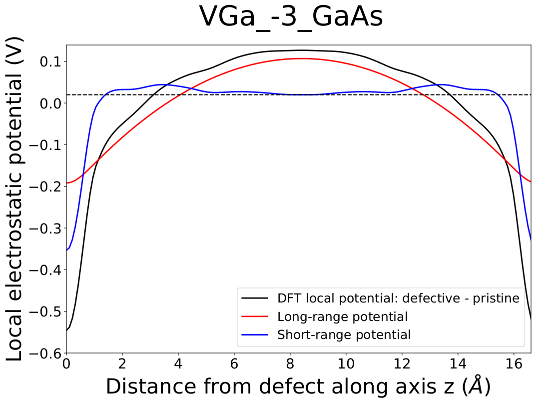
# utility class to plot the electrostatic potential between the defect and
# its image
Plott = fnv.FPlotterPot(axis_grid, dft_potential, lr_potential, sr_potential,
                        -alignment_term, 'z')
# this will save a pdf file called plot_VGa_-3_GaAs.pdf
Plott.plot('VGa_-3_GaAs')

The result of this last block of code is the following picture:

../_images/plot_VGa_-3_GaAs_potentials.png

The scheme of Kumagai and Oba ¶

The keywords arguments for add_correction_scheme_data() are:

Mandatory arguments:

potential_pristine: a 1D array of length equal to the number of atoms in the pristine system. The array elements store the electrostatic potential calculated by first-principles at the atomic sites in the pristine supercell.

potential_defective: a 1D array of length equal to the number of atoms in the defective system. The array elements store the electrostatic potential calculated by first-principles at the atomic sites in the defective supercell.

Optional arguments:

distance_tol: a float or an array with 3 elements. The rounding tolerance for comparing distances. If a float is insert as input, it will be converted to an array of 3 elements. Each element is the tolerance value in percentage of the length of the corresponding cell parameter. The default value is 1% for each cell parameter.

e_tol: a float. The condition for breaking the loop in the iterative calculation of the correction energy. Value in eV. The default value is 1e-6 eV.

Example using VASP ¶

To illustrate in detail how the correction scheme of Kumagai and Oba is implemented in Spinney, we will take the example of a B vacancy in the charge state -3 in cubic BN, modeled using a \(3 \times 3 \times 3\) supercell of the conventional cubic cell. This system is also studied in the authors’ original paper [KO14].

All the data needed by the Kumagai’s and Oba’s scheme are in the OUTCAR file.

The following block of code assumes that the working directory contains the files:

OUTCAR_prist, OUTCAR_def: the OUTCAR files of the pristine and defective supercells, respectively.
OUTCAR_B: the OUTCAR file of the reference state for Boron.

To calculate the defect formation energy with the correction scheme of Kumagai and Oba, you can use this snippet:

import numpy as np

import ase.io
from spinney.io.vasp import extract_potential_at_core_vasp
from spinney.structures.pointdefect import PointDefect

# pristine system
pristine = ase.io.read('OUTCAR_prist')

# Specifications of the defective system: V_B -3 in BN
q = -3 # charge state
e_r = (4.601064 + 2.314707) # electronic and ionic contribution to dielectric
                            # constant, calculated with VASP
a = 0.41667
def_position = np.ones(3)*a # fractional coordinates defect
vbm = 7.2981 # valence band maximum

# Prepare the chemical potentials B-rich conditions
boron = ase.io.read('OUTCAR_B')
mu_b = boron.get_total_energy()/boron.get_number_of_atoms()

# prepare a numpy array with information about the electrostatic potential
pot_prist = extract_potential_at_core_vasp('OUTCAR_prist')
pot_def = extract_potential_at_core_vasp('OUTCAR_def')

# initialite PointDefect instance
defective = ase.io.read('OUTCAR_def')
pd = PointDefect(defective)
pd.set_dielectric_tensor(e_r)
pd.set_defect_position(def_position)
pd.set_defect_charge(q)
pd.set_pristine_system(pristine)
pd.set_vbm(vbm)
pd.set_chemical_potential_values({'N':None, 'B':mu_b}, force=True)
# correction scheme of Kumagai and Oba
pd.set_finite_size_correction_scheme('ko')
pd.add_correction_scheme_data(potential_pristine=pot_prist, potential_defective=pot_def)
print('Formation energy B-rich, uncorrected: {:.3f}'.format(
    pd.get_defect_formation_energy()))
print('Formation energy B-rich, corrected: {:.3f}'.format(
    pd.get_defect_formation_energy(True)))

The script will print:

Formation energy B-rich, uncorrected:  11.801
Formation energy B-rich, corrected:  14.275

Example using WIEN2k ¶

To illustrate in detail how the correction scheme of Kumagai and Oba is implemented in Spinney, we will take the example of a B vacancy in the charge state -3 in cubic BN, modeled using a \(3 \times 3 \times 3\) supercell of the conventional cubic cell. This system is also studied in the authors’ original paper [KO14].

The data that are needed are the .struct, .scf and .vcoul files for the pristine and defective supercell.

Note

By default WIEN2k will not write the .vcoul file. To write it you need to modify the second line of the .in0 file, by replacing NR2V with R2V before running your calculations.

The following block of code assumes that the working directory contains the files:

pristine.struct and defective.struct: the .struct files for the pristine and defective supercell, respectively.
pristine.scf and defective.scf: the .scf files for the pristine and defective supercell, respectively.
pristine.vcoul and defective.vcoul: the .vcoul files for the pristine and defective supercell, respectively.
boron.struct and boron.scf: the .struct and .scf files for the reference state of Boron.

To calculate the defect formation energy with the correction scheme of Kumagai and Oba, you can use this snippet:

import numpy as np

from spinney.structures.pointdefect import PointDefect
from spinney.constants import conversion_table
from spinney.io.wien2k import prepare_ase_atoms_wien2k
from spinney.io.wien2k import extract_potential_at_core_wien2k

# pristine system
pristine = pristine = prepare_ase_atoms_wien2k('pristine.struct',
                                               'pristine.scf')

# Specifications of the defective system: V_B -3 in BN
q = -3 # charge state
e_r = (4.601064 + 2.314707) # electronic and ionic contribution to dielectric
                            # constant
def_position = np.zeros(3) # fractional coordinates defect
vbm = 0.7037187925*conversion_table['Ry']['eV'] # valence band maximum

# Prepare the chemical potentials B-rich conditions
boron = prepare_ase_atoms_wien2k('boron.struct', 'boron.scf')
mu_b = boron.get_total_energy()/boron.get_number_of_atoms()

# prepare a numpy array with information about the electrostatic potential
pot_prist = extract_potential_at_core_wien2k('pristine.struct',
                                             'pristine.vcoul')
pot_prist *= conversion_table['Ry']['eV']
pot_def = extract_potential_at_core_wien2k('defective.struct',
                                           'defective.vcoul')
pot_def *= conversion_table['Ry']['eV']

# initialite PointDefect instance
defective = prepare_ase_atoms_wien2k('defective.struct',
                                     'defective.scf')
pd = PointDefect(defective)
pd.set_dielectric_tensor(e_r)
pd.set_defect_position(def_position)
pd.set_defect_charge(q)
pd.set_pristine_system(pristine)
pd.set_vbm(vbm)
pd.set_chemical_potential_values({'N':None, 'B':mu_b}, force=True)
# correction scheme of Kumagai and Oba
pd.set_finite_size_correction_scheme('ko')
pd.add_correction_scheme_data(potential_pristine=pot_prist, potential_defective=pot_def)
print('Formation energy B-rich, uncorrected: {:.3f}'.format(
    pd.get_defect_formation_energy()))
print('Formation energy B-rich, corrected: {:.3f}'.format(
    pd.get_defect_formation_energy(True)))

The script will print:

Formation energy B-rich, uncorrected: 11.995
Formation energy B-rich, corrected: 14.503

Obtaining more information on the finite-size corrections ¶

More information related to the correction scheme can be accessed through the method calculate_finite_size_correction() with the keyword argument verbose=True.

This returns a tuple, whose first element is the correction energy for finite-size effects and the second element is a dictionary.

The dictionary contains the various contributions to \(E_{corr}\), some information about the sampled atomic-site potential and the instance of the KumagaiCorr` class that has been used to calculate the correction energy term. Such instance can be accessed from the dictionary with the keyword Corr object. From it, we can extract useful information, which allow us, for example to plot the following picture:

../_images/atomic_site_potential_convergence.png

Fig. 4 The picture shows the relevant potentials as a function of the distance from the point defect. Far from the defect the potentials should be relatively flat and smooth. The shaded area represents the sampling region. Potentials that are strongly oscillating in the sampling region indicate that either the supercell is too small, or the defect-induced charge density is not very localized. In either case, convergence of the predicted defect formation energy as a function of the supercell size should be carefully assessed.¶

This image can be obtained using this code snippet. The python interface is independent on the employed first-principles code. We only assume that a PointDefect instance has been initialized, as shown above. Such object is assumed to have been stored in the variable pd. For the meaning of the various potentials plotted in the figure, consult the authors’s paper in reference [KO14].

import matplotlib
import matplotlib.pyplot as plt

matplotlib.rcParams.update({'font.size': 26})

ecorr, dd = pd.calculate_finite_size_correction(verbose=True)
corr_obj = dd['Corr object']

plt.figure(figsize=(8,8))
dist, pot_align_vs_dist = corr_obj.alignment_potential_vs_distance_sampling_region
plt.scatter(dist, pot_align_vs_dist, color='green', marker='^',
            label=r'$\Delta V_{PC, q/b}$')
dist, pot = corr_obj.ewald_potential_vs_distance_sampling_region
plt.scatter(dist, pot, label=r'$V_{PC, q}$', color='blue')
dist, pot = corr_obj.difference_potential_vs_distance
plt.scatter(dist, pot, label=r'$V_{q/b}$', marker='x')
# beginning of the sampling region
radius = corr_obj.sphere_radius
plt.axvspan(radius, 9, color='blue', alpha=0.3)
plt.plot(np.linspace(1.5, 9, 100), np.zeros(100), color='black',
         linestyle='--')
plt.legend()
plt.xlabel(r'Distance ($\AA$)')
plt.ylabel(r'Potential (V)')
plt.xlim(1.5, 9)
plt.ylim(-3, 0.5)
plt.tight_layout()
plt.savefig('atomic_site_potential_convergence.pdf', format='pdf')
plt.show()