Equilibrium defect concentrations in the dilute limit

The formation energy \(\Delta E_f(d; q)\) of a point defect d in charge state q is given by equation (2). In the dilute limit, one assumes non-interacting defects. In this case, the energy required for forming \(n\) defects of type d in charge state q is simply \(n\Delta E_f(d; q)=\Delta E_f(nd; q)\).

At the thermodynamic equilibrium the system grand potential, \(\Phi\), is in a minimum:

(7)\[\Phi(n d; q) = \Phi(\mathrm{bulk}) + \Delta E_f(nd; q) + T S_{conf}(n)\]

where \(S_{conf}\) is the contribution of the configurational entropy to the grand potential of the defective system. Let \(x \equiv (d, q)\) and assume that there are \(g_x\) possible configurations in which defect x has the same \(\Delta E_f(d; q)\) (for example given by spin degeneracy). If the crystal is made of \(N\) unit cell and in each cell there are \(\gamma_x\) equivalent sites that defect x can occupy, the number of possible ways to place \(n\) non-interacting defects on \(N\gamma_x\) sites is (for \(n \ll N\gamma_x\)):

(8)\[\Omega_x = g_x^n \binom{N\gamma_x}{n}\]

from which one gets: \(S_{conf} = k_B \ln \Omega_x\). The equilibrium defect concentration follows from taking the derivative of (7) with respect to \(n\) using Stirling’s approximation for expressing \(S_{conf}\). One gets:

(9)\[c_x = \frac{n}{N} = \frac{\gamma_x g_x}{\exp{\left(\frac{\Delta E_f(d; q)}{k_B T}\right)} + g_x}\]

Usually \(\Delta E_f(d; q) \gg k_B T\) and equation (9) is approximated by:

\[c_x = g_x \gamma_x \exp{\left(-\frac{\Delta E_f(d; q)}{k_B T}\right)}\]

In case of more than one type of defect in the crystal, the equilibrium concentration of each defect is given by formula (9), assuming the dilute-limit holds.

Thermodynamic limits for the chemical potentials explained how Spinney can help in determining the equilibrium values of the atomic chemical potentils in different thermodynamic conditions. The only chemical potential that needs to be determined is the chemical potential of the electron, whose value is fixed by the charge-neutrality constraint:

(10)\[\sum_{x} qc_{x}(\mu_e) + p_0(\mu_e) - n_0(\mu_e) = 0\]

where \(n_0\) is the concentration of free electrons:

\[n_0 = \int_{\epsilon_C}^\infty \frac{\omega(\epsilon) }{e^{(\epsilon - \mu_e)/k_B T} + 1} d\epsilon,\]

and \(p_0\) is the concentration of free holes:

\[p_0 = \int_{-\infty}^{\epsilon_V} \frac{\omega(\epsilon) }{e^{( \mu_e - \epsilon)/k_B T} + 1} d\epsilon.\]

\(\omega(\epsilon)\) is the density of Kohn-Sham states.

Spinney can find \(\mu_e\) by finding the roots of equation (10) from data provided by the user and obtain the equilibrium defect concentrations.

Calculate equilibrium defect concentrations with Spinney

Spinney implements the EquilibriumConcentrations for calculating equilibrium defect concentrations.

The mandatory arguments for initializing a new instance are:

• charge_states: a dictionary mapping each studied defect with the considered charge states.

• form_energy_vbm: a dictionary mapping each studied defect with the formation energies calculated at the valence band maximum for each charge state in charge_states.

• vbm: the value of the valence band maximum used in calculating the defect formation energies recorded in form_energy_vbm.

• e_gap: the calculated band gap.

• site_conc: a dictionary mapping each studied defect with the concentration of available defect sites per unit cell (\(\gamma_x\) of equation (8)). In addition, it maps the concentrations of free holes and electrons. In this case the dictionary keys are hole and electron, respectively.

• dos: a 2D array. The first column reports the energies of the one-electron levels sorted in ascending order; the second column reports the corresponding density of states per simulation cell. The value in dos must be consistent with the values of vbm and e_gap.

• T_range: a 1D array with the temperatures to be used to calculate the defect concentration.

Optional arguments are:

• g: a dictionary mapping each studied defect with its degeneracy for each charge state in charge_states.

• N_eff: a number indicating an effective doping concentration. Its value will affect the calculated value of the equilibrium electron chemical potential using the equation:

\[\sum_{x} qc_{x}(\mu_e) + p_0(\mu_e) - n_0(\mu_e) = N_{eff}\]

• units_energy: the units of energy that are used, by default eV are used.

• dos_down: for spin-polarized systems, the DOS of spin-down electrons. Data structure completely analogous to dos.

We will use as an example the intrinsic defects in GaN, considered also in Manage a defective system with the class DefectiveSystem and in Charge Transition Levels.

charge_states   = {'N_Ga'   : [-1, 0, 1, 2, 3],
                   'Ga_int' : [0, 1, 2, 3],
                   'Ga_N'   : [-1, 0, 1, 2, 3],
                   ...
                  }

form_energy_vbm = {'N_Ga'   : [11.0872728320, 8.2717122490, ...],
                   'Ga_int' : [8.3391662537, 5.1149599825, ...],
                   'Ga_N'   : [8.1902691783, 5.5148367310, ...],
                   ...
                  }

Indicating, for example, that the formation energy, for an electron chemical potential equal to the valence band maximum, of a Ga interstitials in charge state +1 is 5.1149599825 eV. The names used to indicate the various type of point defects must be consistent with each other. Such data structures can be easily obtained from the text file produced by DefectiveSystem using the method write_formation_energies(), which have the format shown in Step 2: Get Thermodynamic Charge Transition Levels and plot the Diagram.

So as a first step, one calculates the defect formation energies for the various point defects of interest, for example using a DefectiveSystem object. As done in previous section we consider in this example the Ga-rich limit:

import os

import ase.io
from spinney.structures.defectivesystem import DefectiveSystem
from spinney.tools.formulas import count_elements

path_defects = os.path.join('data', 'data_defects')
path_pristine = os.path.join('data', 'pristine', 'OUTCAR')
path_ga = os.path.join('data', 'Ga', 'OUTCAR')

ase_ga = ase.io.read(path_ga, format='vasp-out')

# Band alignment
vbm_offset = 0.85
vbm = 5.009256 - vbm_offset # align the VBM with the HSE band
e_gap = 1.713
# dielectric tensor
e_rx = 5.888338 + 4.544304
e_rz = 6.074446 + 5.501630
e_r = [[e_rx, 0, 0], [0, e_rx, 0], [0, 0, e_rz]]

# get the chemical potential of Ga
ase_pristine = ase.io.read(path_pristine, format='vasp-out')
chem_pot_ga = ase_ga.get_total_energy()/ase_ga.get_number_of_atoms()
# get the chemical potential of N in the Ga-rich conditions
elements = count_elements(ase_pristine.get_chemical_formula())
chem_pot_n = ase_pristine.get_total_energy() - elements['Ga']*chem_pot_ga
chem_pot_n /= elements['N']

# initialize a DefectiveSystem
defective_system = DefectiveSystem('data', 'vasp')
defective_system.vbm = vbm
defective_system.dielectric_tensor = e_r
defective_system.chemical_potentials = {'Ga':chem_pot_ga, 'N':chem_pot_n}
defective_system.correction_scheme = 'ko'
defective_system.calculate_energies(verbose=False)
# write the defect formation energies in a text file
defective_system.write_formation_energies('formation_energies_GaN_Ga_rich.txt')

Note that in:

# Band alignment
vbm_offset = 0.85
vbm = 5.009256 - vbm_offset # align the VBM with the HSE band
e_gap = 1.713

we have lowered the PBE valence band maximum by 0.85 eV in order to align it with the valence band value obtained using a hybrid functional (see Charge Transition Levels). This will lower the formation energies of positive charge states by \(q \times 0.85\) and increase those of negative states by \(|q| \times 0.85\). So aligning the valence band maximum will have considerable effects on the defect formation energies.

charge_states and form_energy_vbm can be obtained from the text file formation_energies_GaN_Ga_rich.txt calling the function extract_formation_energies_from_file() in the module concentration. The function takes as the only argument the text file with the defect formation energies and returns the dictionaries to be used as the parameters charge_states and form_energy_vbm of EquilibriumConcentrations:

from spinney.defects.concentration import extract_formation_energies_from_file

energy_file = 'formation_energies_GaN_Ga_rich.txt'
charge_states, form_energy_vbm = extract_formation_energies_from_file(energy_file)

We can now process the rest of the data:

• vbm will be equal to the shifted valence band maximum: vbm = 5.009256 - vbm_offset.

Warning

vbm is the valence band maximum of the unit cell used to calculate dos. In GaN, the valence band maximum is located at the \(\Gamma\) point and the valence band eigenvalues of the primitive and pristine supercell are basically the same. For other materials, the values could differ. It is important that vbm and dos are always consistent with each other.

• e_gap is directly obtained from the output of first-principles calculations. Here we use the value predicted by PBE for the primitive cell.

• site_conc can be determined for example by looking at the multiplicities of the Wyckoff position of the site where the point defect sits. In the wurtzite structure, the Wyckoff position for both Ga and N is \((2b)\). Considering the primitive cell as reference cell, one would have:

site_conc = {'Ga_N':4, 'N_Ga':4, 'Vac_N':4, 'Vac_Ga':4,
             'Ga_int':6, 'N_int':6, 'electron':36 , 'hole':36}

the site symmetry of the interstitial atoms is compatible with the \((6c)\) Wyckoff position. For electron and holes we used the number of valence electrons per primitive cell. Using such site_conc in initializing EquilibriumConcentrations would make the code calculate defect concentrations per primitive cell. One usually reports defect concentrations in \(cm^{-3}\). So, for GaN, whose equilibrium volume at the PBE level is 47.04 \(\AA^{3}\), one needs to multiply the values in site_conc by 2.126e+22 in order to obtain concentrations in \(cm^{-3}\).

• dos can be straightforwardly obtained from the first-principles calculations. However, in our example we need to modify it. For one, we have to shift the valence band maximum in the first column of dos by -0.85 eV, so that it agrees with vbm. If dos has been read and stored to a 2D numpy array, such operation is trivial:

dos[:, 0] -= vbm_offset

• T_range can be chosen to be any array of interest. We can calculate defect concentrations from 250 K to 1000 K taking 100 sampling points:

T_range = np.linspace(250, 1000, 100)

A instance of EquilibriumConcentrations can now be initialized:

concentrations = EquilibriumConcentrations(charge_states, form_energy_vbm,
                                           vbm, e_gap, site_conc, dos, T_range)

Equilibrium properties of the system can now be calculated an accessed through the instance attributes:

• concentrations.equilibrium_fermi_level: returns a Numpy array with len(T_range) elements, with the calculated equilibrium value of the electron chemical potential as a function of the input temperature. concentrations.equilibrium_fermi_level - concentrations.vbm can be used to obtain the Fermi level with respect to the valence band maximum.

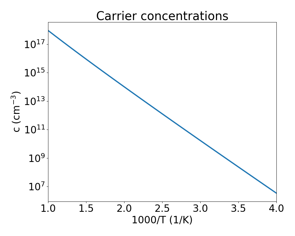
The picture shows that intrinsic GaN is a n-type semiconductor and that the carrier concentration will increase as the temperature increases.

• concentrations.equilibrium_carrier_concentrations returns a Numpy array with the equilibrium carrier concentrations as a function of the temperature. The quantity returned is the difference between hole and electron concentrations. For intrinsic GaN the signs are negative, indicating that electrons are indeed the majority carriers. The plot below shows the absolute value of concentrations.equilibrium_carrier_concentrations as a function of \(1000/T\). Note that the electron concentration will be largely overestimated as we have used the PBE band gap, which is much smaller than the experimental one. Opening the gap, e. g. by applying a scissor operator, might change the calculated concentrations by order of magnitudes.

• concentrations.equilibrium_defect_concentrations returns a dictionary, where each key is the name of the point defect, as used in charge_states and form_energy_vbm. The values are other dictionaries, where the keys are the defect charge state and the value a Numpy array with the defect concentrations as a function of the temperature.

For example, the equilibrium defect concentrations of nitrogen vacancies, which we indicated using Vac_N, in the charge state +2 can be obtained from: concentrations.equilibrium_defect_concentrations['Vac_N'][2].

The picture shows that the majority carriers originate from the ionization of donor-type N vacancies, which have a low formation energy, as shown in Fig. 8 of section Charge Transition Levels.

For convenience and for allowing further processing of defect concentrations, an EquilibriumConcentrations instance also collects the data in a Pandas DataFrame object, accesible through the attribute defect_concentrations_dataframe.

df = concentrations.defect_concentrations_dataframe
# the temperature is used for the row labels
df.loc[500] # Panda Series with formation energies at 500K

Equilibrium concentrations for free electrons and holes as a function of the temperature can be accessed through the attributes equilibrium_electron_concentrations and equilibrium_holes_concentrations, respectively. A Pandas DataFrame with the equilibrium carrier concentrations is given by the attribute carrier_concentrations_dataframe.

carriers_df = concentrations.carrier_concentrations_dataframe
# merge data frames for further processing
import pandas as pd
new_df = pd.concat([df, carriers_df], axis=1)
# show that free electron are almost entirely generated by single ionization of Vac_N
data = new_df.loc[:, [('Vac_N', 1), 'electron']].values
plt.plot(T_range, (data[:, 1] - data[:, 0])/data[:, 1])
plt.show()

Through this last snippet, the curve reproduced in the below image is obtained, which shows that more than 99% of free electrons are due to the single ionization of nitrogen vacancies.

Using the class DefectiveSystem

Using the usual directory structure we can prepare an DefectiveSystem instance and access an EquilibriumConcentrations object from it.

The following code snippet will prepare an instance of the class DefectiveSystem, calculate the defect formation energies in the Ga-rich limit and produce an EquilibriumConcentrations instance, which can be accessed through the attribute concentrations of the DefectiveSystem instance. Such EquilibriumConcentrations instance can be used as shown in the previous section to obtain equilibrium defect and carriers concentrations as a function of the temperature.

import numpy as np
import os
import ase.io
from spinney.structures.defectivesystem import DefectiveSystem
from spinney.tools.formulas import count_elements
from spinney.io.vasp import extract_dos

path_defects = os.path.join('data', 'data_defects')
path_pristine = os.path.join('data', 'pristine', 'OUTCAR')
path_ga = os.path.join('data', 'Ga', 'OUTCAR')

ase_ga = ase.io.read(path_ga, format='vasp-out')

# Band alignment
vbm_offset = 0.85
vbm = 5.009256 - vbm_offset # align the VBM with the HSE band
e_gap = 1.713

# dielectric tensor
e_rx = 5.888338 + 4.544304
e_rz = 6.074446 + 5.501630
e_r = [[e_rx, 0, 0], [0, e_rx, 0], [0, 0, e_rz]]

# get the chemical potential of Ga
ase_pristine = ase.io.read(path_pristine, format='vasp-out')
chem_pot_ga = ase_ga.get_total_energy()/ase_ga.get_number_of_atoms()
# get the chemical potential of N in the Ga-rich conditions
elements = count_elements(ase_pristine.get_chemical_formula())
chem_pot_n = ase_pristine.get_total_energy() - elements['Ga']*chem_pot_ga
chem_pot_n /= elements['N']

# get the density of states
dos = extract_dos('vasprun.xml')[0]
dos [:,0] -= vbm_offset

# site concentrations for point defects
volume = ase_pristine.get_volume()/ase_pristine.get_number_of_atoms()
volume *= 4
factor = 1e-8**3 * volume
factor = 1/factor
site_conc = {'Ga_N':4, 'N_Ga':4, 'Vac_N':4, 'Vac_Ga':4,
             'Ga_int':6, 'N_int':6, 'electron':36 , 'hole':36}
site_conc = {key:value*factor for key, value in site_conc.items()}

defective_system = DefectiveSystem(os.path.join('..', 'diagram', 'data'),
                                   'vasp')
defective_system.vbm = vbm
defective_system.dielectric_tensor = e_r
defective_system.chemical_potentials = {'Ga':chem_pot_ga, 'N':chem_pot_n}
defective_system.correction_scheme = 'ko'
# specific data for obtaining the EquilibriumDefectConcentration object
defective_system.gap_range = (vbm, vbm + e_gap)
defective_system.site_concentrations = site_conc
defective_system.temperature_range = np.linspace(250, 1000, 100)
defective_system.dos = dos
defective_system.calculate_energies(False)

# EquilibriumDefectConcentrations object
concentrations = defective_system.concentrations