Thermodynamic limits for the chemical potentials

The defect formation energy of equation (2) explictly depends on the chemical potentials of the elements which are exchanged with the reservoir in order to introduct the point defect.

The thermodynamic stability of the host crystal imposes some constraints on the values these chemical potentials can assume.

Consider for example the rutile phase of \(\mathrm{TiO_2}\). If \(\mu_i\) represents the chemical potential of element \(i\) and \(\Delta \mu_i\) represents its value with respect to the element chemical potential in its standard state (say the HCP structure for Ti and the triplet state of the \(\mathrm{O_2}\) molecule for O), the following constraint have to be satisfied:

\begin{align*} \mu_\mathrm{Ti} + 2\mu_\mathrm{O} &= \mu_\mathrm{TiO_2(rutile)}\\ x\mu_\mathrm{Ti} + y\mu_\mathrm{O} &\leq \mu_\mathrm{Ti_xO_y}\\ \mu_\mathrm{Ti} &\leq \mu_\mathrm{Ti(HCP)}\\ \mu_\mathrm{O} &\leq \frac{1}{2} \mu_\mathrm{O_2} \end{align*}

Or equivalently:

\begin{align*} \Delta \mu_\mathrm{Ti} + 2\Delta \mu_\mathrm{O} &= \Delta h_\mathrm{TiO_2(rutile)}\\ x\Delta \mu_\mathrm{Ti} + y\Delta \mu_\mathrm{O} &\leq \Delta h_\mathrm{Ti_xO_y}\\ \Delta \mu_\mathrm{Ti} &\leq 0\\ \Delta \mu_\mathrm{O} &\leq 0 \end{align*}

where \(\Delta h\) is the formation enthalpy per formula unit.

Limiting values of the chemical potentials

Defect formation energies are usually reported for the extreme conditions; in this case:

• O-rich conditions, where \(\mu_\mathrm{O}\) achieves its maximum value;

• Ti-rich conditions, where \(\mu_\mathrm{Ti}\) achieves its maximum values.

Such values can be obtained from the solution of the optimization problem of equation (5) or (6).

Spinney offers the Range class for this purpose.

Suppose that the formation energies per formula unit of the relevant Ti-O phases have been calculated and written on a text file, formation_energies.txt like the one below:

# Formation energies per formula unit calculated with PBEsol
#Compound                 E_f (eV/fu)
Ti                          0.0000000000
O2                          0.0000000000
TiO2_rutile                -9.4742301250
Ti2O3                     -15.2633270550
TiO                        -5.3865639660
Ti3O5                     -24.8910858875

The problem in equation (5) can be solved creating an instance of the Range class.

The data needed by this class can be obtained from a text file analogous to the one above using the function get_chem_pots_conditions().

This function takes four arguments:

• The text file with the calculated formation energies. get_chem_pots_conditions() assumes that each row represents either the formation energies per formula unit calculated for a compound with respect to its elements in the standard state, or the total energy of the compound, again per formula unit.

  Comments can be added by starting a line with #.

  Each line containing the energy data must have the form: compound_name<delimiter>energy. compound_name must be a string containing the formula unit of the compound. Underscores can then be added to separate other strings. <delimiter> is a string that divides compound_name and energy. By default blank spaces are assumed. energy is a string representing a floating-point number.

• A list specifying the order of the variables (that is, the chemical elements).

• A list with all the compound_name in the text file that represent compounds characterized by an equality constraint.

• (Optional) A string that specifies <delimiter> used in the text file.

The returned values can be used to initialize the Range class and some of its methods, like shown in the example below:

from spinney.thermodynamics.chempots import Range, get_chem_pots_conditions

data = 'formation_energies.txt'

equality_compounds = ['TiO2_rutile']
order = ['O', 'Ti']
parsed_data= get_chem_pots_conditions(data, order, equality_compounds)
# prepare Range instances
crange = Range(*parsed_data[:-1])

The minimum and maximum value that each variable (chemical potential) can obtain within the feasible region can by accessed through the attribute variables_extrema of the class Range. This returns a 2D array, with \(n\) rows and \(2\) columns, with n being the number of variables in equation (5). Each row gives the minimum and maximum value of one variable, the order is the same we specified in order.

For example, typing:

print(crange.variables_extrema)

returns:

array([[-3.53160448e+00, -8.94320056e-14],
       [-9.47423008e+00, -2.41102114e+00]])

The first row is relative to \(\Delta \mu_\mathrm{O}\) and indicates that this variable can range between -3.53 eV and 0 eV. The end point of this interval represent the value of \(\Delta \mu_\mathrm{O}\) in the Ti-rich and O-rich limit, respectively.

One can see that \(\Delta \mu_\mathrm{Ti}\) has a maximum value of -2.41 eV (Ti-rich limit), meaning that thermodynamic equilibrium between rutile and Ti is not possible.

Plotting the feasible region

Competing phases can be easily visualized by plotting the feasible region. This can be done in Spinney adding this code snippet to the previous script:

range.set_compound_dict(parsed_data[-1])
# let's use some pretty labels in the plot
# the order of the axes  must follow the order used for get_chem_pots_conditions
labels = [r'$\Delta \mu_{O}$ (eV)', r'$\Delta \mu_{Ti}$ (eV)']
crange.plot_feasible_region_on_plane([0,1], x_label=labels[0],
                                     y_label=labels[1],
                                     title='Rutile phase', save_plot=True)

Which saves the plot in the pdf file feasible_region_plane_0_1.pdf:

The feasible region has been intersected with the 0-1 plane, which is the plane spanned by the independent chemical potentials. The ordering of these is the one that has been specified in order. In our example the variable 0 is \(\Delta \mu_\mathrm{O}\) and variable 1 is \(\Delta \mu_\mathrm{Ti}\). If instead we would have used [1, 0] as the first argument of range.plot_feasible_region_on_plane, we would have obtained a plot with switched axes, saved as feasible_region_plane_1_0.pdf

This plot represents the feasible region for the problem described by equation (5). In particular, the shaded area is the feasible region determined by the inequality constratints and the black line is determined by the equality constraint. Such plots offer a convenient way to visualize the relevant competing phases for given values of the element chemical potentials.

From the picture it is clear that \(\mathrm{Ti_3O_5}\) would precipitate before the chemical potential of Ti reaches its standard state value.

Warning

A PointDefect object takes the absolute values of the chemical potentials in order to calculate the defect formation energy. These can be obtained from \(\Delta \mu\) by adding to it the chemical potential of the standard state. Equivalently, these values can be obtained by using equation (5) instead of equation (6) by modifying the file formation_energies.txt accordingly.

Beyond binary compounds

Suppose we now want to consider rutile doped with Nb. We consider as a possible competing phase \(\mathrm{TiNb_2O_7}\) and \(\mathrm{NbO_2}\) (other compounds could be considered of course).

The file formation_energies.txt is modified accordingly and renamed formation_energies_with_nb.txt:

# Formation energies per formula unit calculated with PBEsol
#Compound                 E_f (eV/fu)
Ti                          0.0000000000
O2                          0.0000000000
TiO2_rutile                -9.4742301250
Ti2O3                     -15.2633270550
TiO                        -5.3865639660
Ti3O5                     -24.8910858875
TiNb2O7                   -28.9191827617
Nb                          0.0000000000
NbO2                      -8.06605626125

To instantiate the proper Range object, one can type:

data_nb = 'formation_energies_with_nb.txt'

equality_compounds = ['TiO2_rutile']
order = ['O', 'Ti', 'Nb'] # must insert the new species
parsed_data= get_chem_pots_conditions(data_nb, order, equality_compounds)
# prepare Range instances
crange_nb = Range(*parsed_data[:-1])

crange_nb.set_compound_dict(parsed_data[-1])
labels = [r'$\Delta \mu_{O}$ (eV)', r'$\Delta \mu_{Ti}$ (eV)', r'$\Delta \mu_{Nb}$ (eV)']

We can now plot the feasible region on the O-Ti plane. Since we have an additional variable, we must specify the value of \(\Delta \mu_{\mathrm{Nb}}\) that defines the plane intersecting the feasible region. We can do so by using the argument plane_values of plot_feasible_region_on_plane(). This is a list and specifies the values of the variables which are not used as independent variables in the plot.

We can for example consider Nb-rich conditions, where \(\Delta \mu_\mathrm{Nb} = 0\). So that the independent variables are \(\Delta \mu_\mathrm{O}\) and \(\Delta \mu_\mathrm{Ti}\). To plot the intersection of the feasible region with the plane \(\Delta \mu_\mathrm{Nb} = 0\). of the 3D \(\Delta \mu_\mathrm{O}\)-\(\Delta \mu_\mathrm{Ti}\)-\(\Delta \mu_\mathrm{Nb}\) space we set plane_axes=[0,1] and plane_values=[0]:

crange_nb.plot_feasible_region_on_plane([0, 1], x_label=labels[0],
                                        y_label=labels[1],
                                        plane_values = [0],
                                        y_val_min = -10, # minimum value second variable
                                        title='Rutile phase, Nb doping, Nb-rich',
                                        save_plot=True,
                                        save_title='feasible_region_Nb_rich')

This snippet will save a pdf file called feasible_region_Nb_rich.pdf:

From the feasible region it is clear that for Nb-rich conditions (\(\Delta \mu_\mathrm{Nb} = 0\)) rutile would not be thermodynamically stable, as \(\mathrm{NbO_2}\) would precipitate instead.

We could instead ask for which value of \(\Delta \mu_\mathrm{Nb}\) rutile would be stable in O-rich (\(\Delta \mu_\mathrm{O} = 0\)) conditions. To do so, we itersect the feasible region with the plane \(\Delta \mu_\mathrm{O} = 0\) by setting plane_axes=[1, 2] and plane_values=[0].

crange_nb.plot_feasible_region_on_plane([1, 2], x_label=labels[1],
                                        y_label=labels[2],
                                        plane_values = [0],
                                        title='Rutile phase, Nb doping, O-rich', save_plot=True,
                                        save_title='feasible_region_O_rich')

The snippet will produce the picture:

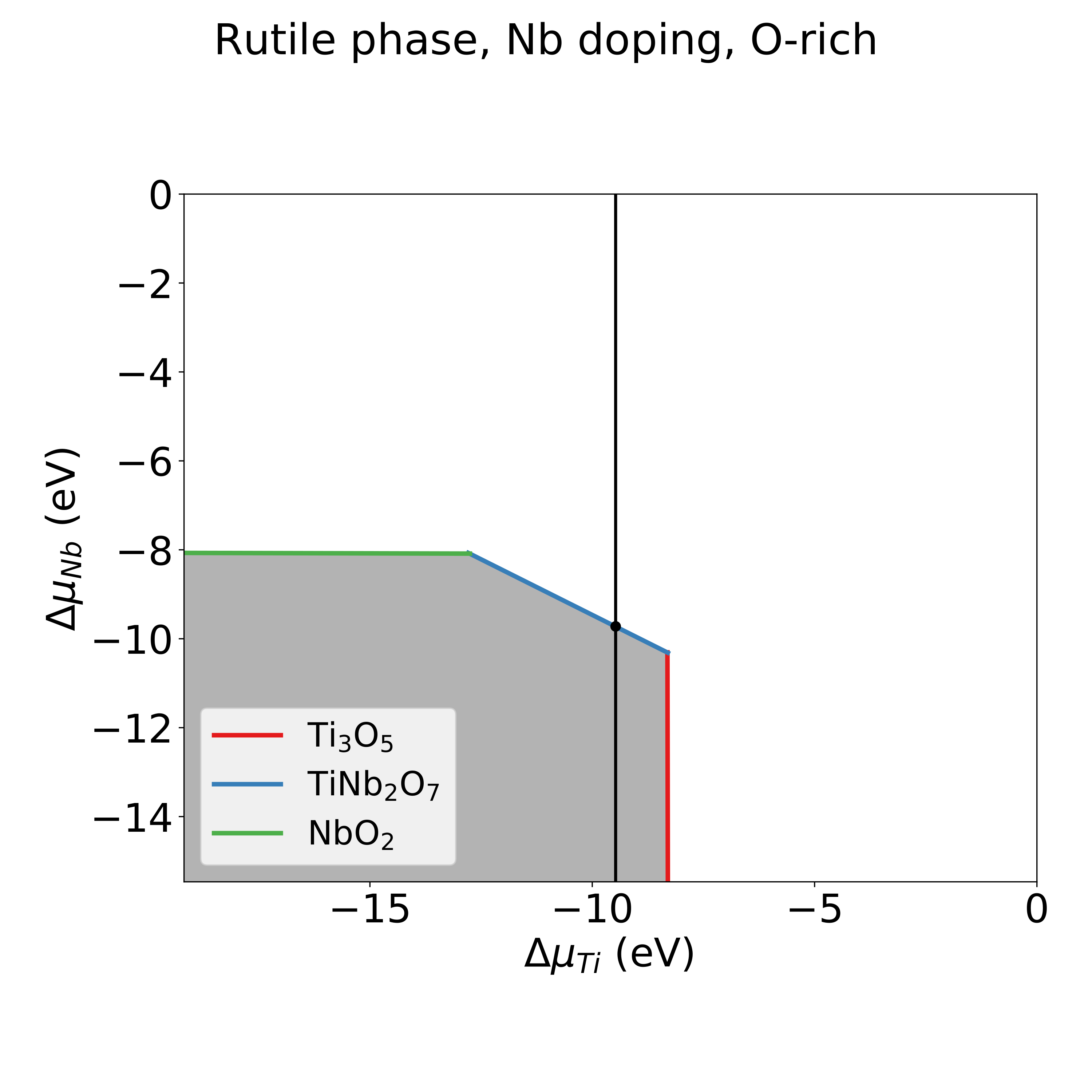
We can see that the maximum value of \(\Delta \mu_\mathrm{Nb}\) compatible with the stability of rutile in oxygen-rich conditions is determined by the formation of \(\mathrm{TiNb_2O_7}\). Using the class attribure variables_extrema_2d one can have access to this value. The attribute is defined analogously as variables_extrema, but considers the optimization problem after the intersection has been considered and refers to the two independent variables defining the plane axes, \(\Delta \mu_\mathrm{Ti}\) and \(\Delta \mu_\mathrm{Nb}\) in this case.

print(crange_nb.variables_extrema_2d)

prints:

[[-9.47423013 -9.47423013]
 [       -inf -9.72247632]]

The second row of the array corresponds to \(\Delta \mu_\mathrm{Nb}\) and shows that its maximum value compatible with the existance of rutile when \(\Delta \mu_\mathrm{O} = 0\) is around -9.72 eV. At this point both \(\Delta \mu_\mathrm{Nb}\) and \(\Delta \mu_\mathrm{O}\) are fixed, there are then no more degrees of freedom and \(\Delta \mu_\mathrm{Ti}\) can only have a single value which is fixed by the constraint of coexistance between rutile and \(\mathrm{TiNb_2O_7}\).

Including temperature and pressure effects through the gas-phase chemical potentials

Spinney implements, for the common gas species \(\mathrm{O}_2\), \(\mathrm{H}_2\), \(\mathrm{N}_2\), \(\mathrm{F}_2\), and \(\mathrm{Cl}_2\), conventient expressions for calculating the chemical potentials as a function of temperature and pressure. It uses the following formula, based on the Shomate equation [MWC98] and an ideal gas model:

\[\mu(T, p) = h(0, p^\circ) + [g(T, p^\circ) - g(0, p^\circ)] + k_BT\ln\left(\frac{p}{p^\circ}\right)\]

\(p^\circ\) represents the standard pressure of 1 bar, \(g\) the molar free energy and \(h(0, p^\circ)\) the molar enthalpy at zero temperature and standard pressure.

For example, consider the case of \(\mathrm{O}_2\). In this case we would use the class OxygenChemPot class. For each of the above-mentioned species there is an analogous class whose construct takes two arguments: the unit of energy used to return \(\mu\) and the unit of pressure. Valid units can be found in the variable spinney.constants.available_units:

available_units = ['J', 'eV', 'Ry', 'Hartree', 'kcal/mol', 'kJ/mol',
                   'm', 'Angstrom', 'Bohr', 'nm', 'cm',
                   'Pa', 'kPa', 'Atm', 'Torr']

For \(\mathrm{O}_2\):

from spinney.thermodynamics.chempots import OxygenChemPot

o2 = OxygenChemPot(energy_units='eV', pressure_units='Atm')

We can now use the method get_ideal_gas_chemical_potential_Shomate() to obtain the chemical potential values as a function of temperature and pressure. The signature of this method is:

get_ideal_gas_chemical_potential_Shomate(mu_standard, partial_pressure, T)

mu_standard is a scalar, representing \(h(0, p^\circ)\). It can be set equal to the electronic energy calculated for the molecule, alternatively, in this example we will set it to zero, in such a way we would obtain \(\Delta \mu_{O_2}\), that is the difference from the reference state.

Both partial_pressure and T can be either scalars or 1-dimensional arrays.

For example, this snippet will plot \(\Delta \mu_{O_2}\) as a function of temperature for \(p = 1\) Atm.

Note

The Shomate equation is valid only for some values of T, if the input values are not in this range, a ValueError will be raised. The exception message will indicate the possible temperature range for that gas species.

import numpy as np
import matplotlib.pyplot as plt

from spinney.thermodynamics.chempots import OxygenChemPot

o2 =  OxygenChemPot(energy_units='eV', pressure_units='Atm')

T_range = np.linspace(300, 1000, 200)
chem_pot_vs_T = o2.get_ideal_gas_chemical_potential_Shomate(0, 1, T_range)

plt.plot(T_range, chem_pot_vs_T, linewidth=2)
plt.xlabel('T (K)')
plt.ylabel(r'$\Delta \mu_{O_2}$ (eV)')
plt.show()

And this snippet will plot the same graph but at tree different pressures:

import numpy as np
import matplotlib.pyplot as plt

from spinney.thermodynamics.chempots import OxygenChemPot

o2 =  OxygenChemPot(energy_units='eV', pressure_units='Atm')

T_range = np.linspace(300, 1000, 200)
pressures = [1, 10, 1e-6]
chem_pot_vs_T = o2.get_ideal_gas_chemical_potential_Shomate(0, pressures, T_range)

plt.plot(T_range, chem_pot_vs_T, linewidth=2)
plt.legend([str(p) + ' Atm' for p in pressures])
plt.xlabel('T (K)')
plt.ylabel(r'$\Delta \mu_{O_2}$ (eV)')
plt.show()