Case Study: Mg-doped GaN
This tutorial will show how to calculate the main quantities of interest for a defective system using Spinney. It is meant to offer a quick overview of the capabilities of Spinney and how to use the code in practice. For a more detailed guide, see the full Tutorial.
We will take as an example Mg-doped GaN. GaN is a material which is extensevely employed in several devices. It shows an intrinsic \(n\)-type conductivity; on the other hand, the ability of synthesizing \(p\)-type GaN would be very beneficial for many technological applications such as optoelectronic devices. Obtaining \(p\)-type carriers is very challenging and Mg is arguably the only dopant that has been successfully employed in the synthesis of \(p\)-type GaN.
Contents
Step 1. Defining the values of chemical potentials
Important quantities that characterize a defective system, such as defect formation energies are affected by the chemical potential values of the elements forming the defective system.
The thermodynamic stability of the host material imposes some constraints on the values these chemical potentials can assume.(For more details see the dedicated session in the main tutorial).
For the case of Mg-doped GaN, let \(\Delta \mu_i\) represents the value of the chemical potential of element \(ì\) from the element chemical potential in its standard state (crystalline orthorhombic phase for Ga, \(\mathrm{N}_2\) molecule for N and the crystalline HCP phase for Mg). The thermodynamic stability of GaN requires that the following constraints are satisfied:
where \(\Delta h\) is the formation enthalpy per formula unit.
For calculating physically acceptable values for the chemical potentials, we can use the Range class.
It is useful to prepare a text file, for example called formation_energies.txt which for each compound in the Ga-N-Mg system reports in the first column the compound formula unit and in the second column its formation energy per formula unit. In our example we can use:
# Formation energies per formula unit calculated with PBE for GaN
#Compound                 E_f (eV/fu)
MgGa2                     -0.3533064287
Mg3N2                     -3.8619941875
Mg2Ga5                    -0.7160803263
Ga                         0.0000000000
Mg                         0.0000000000
GaN                       -0.9283419463
N                          0.0000000000
Line starting with # are comments and will be skipped, more compounds can of course be consider, but we limit ourselves to few of them for simplicity.
The following snippet of code shows the minimum and maximum value that \(\Delta \mu_i\) can assume in order to satisfy the constraints (1).
from spinney.thermodynamics.chempots import Range, get_chem_pots_conditions

data = 'formation_energies.txt'

equality_compounds = ['GaN'] # compound where the constraint is an equation
order = ['Ga', 'N', 'Mg'] # chemical potential 0 is for Ga, 1 for N etc
# obtain data to feed to the Range class
parsed_data= get_chem_pots_conditions(data, order, equality_compounds)
# prepare Range instances
crange = Range(*parsed_data[:-1])

# for each chemical potential, stores the minimum and maximum possible values
ranges = crange.variables_extrema
print(ranges)
Output:
[[-9.28341946e-01 -2.21944834e-14]
 [-9.28341946e-01 -3.94026337e-14]
 [           -inf -6.68436765e-01]]
In principle both \(\Delta \mu_\mathrm{Ga}\) and \(\Delta \mu_\mathrm{N}\) can range from \(h_\mathrm{GaN}\) to 0. Clearly the value of one chemical potential fixes the other as given by equation (1).
Suppose we are interested in GaN growth in Ga-rich conditions. We want then set \(\Delta \mu_\mathrm{Ga}= 0\). We need to find acceptable values for \(\Delta \mu_\mathrm{N}\) and \(\Delta \mu_\mathrm{Mg}\). The former is fixed once \(\Delta \mu_\mathrm{Ga}\) is fixed. For the latter, it is usually observed that high concentrations of Mg are needed to fabricate \(p\)-type GaN. We would then like to consider conditions in which the chemical potential of Mg is as close as possible to the one of pure metal Mg.
We can investigate the acceptable values of \(\Delta \mu_\mathrm{Mg}\) by plotting the intersection of the feasible region with the plane \(\Delta \mu_\mathrm{Ga}= 0\), and print the mimimum and maximum value the chemical potential can assume on this plane, as shows this code snippet:
# compound labels
crange.set_compound_dict(parsed_data[-1])
# let's use some pretty labels in the plot
# the order of the axes  must follow the order used for get_chem_pots_conditions
labels = [r'$\Delta \mu_{Ga}$ (eV)', r'$\Delta \mu_{N}$ (eV)',
          r'$\Delta \mu_{Mg}$ (eV)']
# intersection plane is defined by axes 1 and 2 (chem pot of N and Mg)
crange.plot_feasible_region_on_plane([1,2], x_label=labels[1],
                                     y_label=labels[2],
                                     title='GaN Ga-rich',
                                     save_plot=True)
# chemical potential boundaries on such plane
print(crange.variables_extrema_2d)
Output:
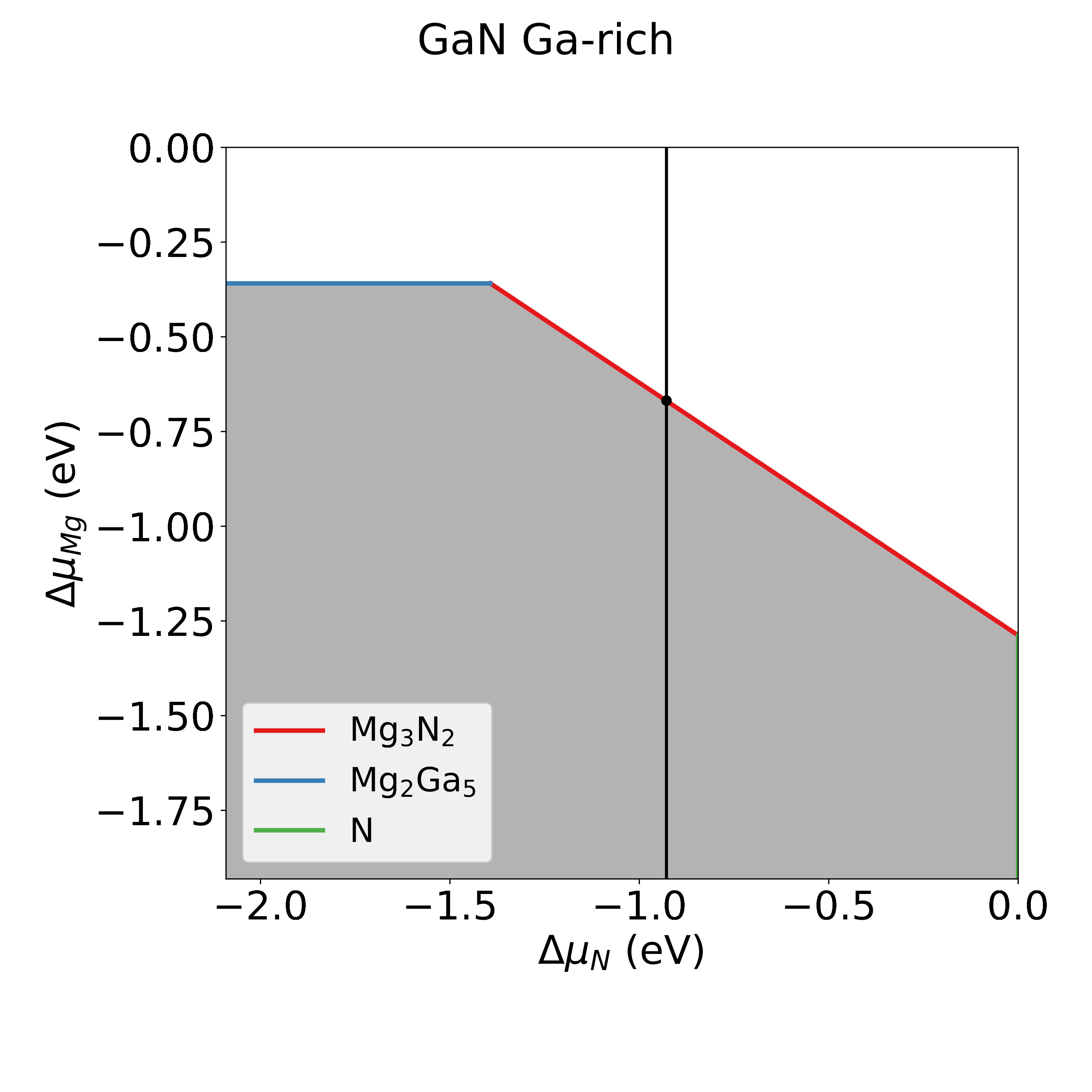
[[-0.92834195 -0.92834195]
 [       -inf -0.66843676]]
The shaded are in the plot show the feasible region corresponding to the inequality constraints of equation (1). From the plot it is clear that \(\Delta \mu_\mathrm{Mg}\) can assume a maximum value of -0.668 eV. It is not possible to go to Mg-richer conditions as \(\mathrm{Mg_3N_2}\) would start to precipitate.
In the study of defective Mg-doped GaN we will then consider the chemical potentials:
\(\Delta \mu_\mathrm{Ga} = 0\)
\(\Delta \mu_\mathrm{N} = \Delta h_\mathrm{GaN}\)
\(\Delta \mu_\mathrm{Mg} = -0.668\)
Corresponding to a system in equilibrium with pure Ga and \(\mathrm{Mg_3N_2}\).
Step 2. Set up the directory with the data about the defective system
Once we have an idea about the thermodynamic stability of the system, we can run the calculations of the defective system.
Most of the properties of interest of a defective system depend on the energy of the system with a point defect and pristine system. It is convenient to save the results of our calculations using the directory hierarchy understood by Spinney.
We will consider that all the calculations have been performed with the code VASP (for details when other codes are used see Manage a defective system with the class DefectiveSystem). Calculations have been performed at the PBE level using supercells with 96 atoms.
The directory tree might look like this:
data
├── data_defects
│   ├── Ga_int
│   │   ├── 0
│   │   │   ├── OUTCAR
│   │   │   └── position.txt
│   │   ├── 1
│   │   │   ├── OUTCAR
│   │   │   └── position.txt
│   │   ├── 2
│   │   │   ├── OUTCAR
│   │   │   └── position.txt
│   │   └── 3
│   │       ├── OUTCAR
│   │       └── position.txt
│   ├── Ga_N
│   │   ├── 0
│   │   │   ├── OUTCAR
│   │   │   └── position.txt
│   │   ├── 1
│   │   │   ├── OUTCAR
│   │   │   └── position.txt
│   │   ├── -1
│   │   │   ├── OUTCAR
│   │   │   └── position.txt
│   │   ├── 2
│   │   │   ├── OUTCAR
│   │   │   └── position.txt
│   │   └── 3
│   │       ├── OUTCAR
│   │       └── position.txt
...
├── Ga
│   └── OUTCAR
├── N2
│   └── OUTCAR
├── Mg
│   └── OUTCAR
└── pristine
    └── OUTCAR
For the study of Mg-doped GaN, we are considering the intrinsic defects as well, as these will always be present and will affect the properties of the doped system.
Initialize an DefectiveSystem instance
The easiest way to process the calculations of point defects is through the class
DefectiveSystem.
from spinney.structures.defectivesystem import DefectiveSystem
# initialize the defective system, where calculations have been done with VASP
defective_system = DefectiveSystem('data', 'vasp')
Once the object has been initialized, we can use it to compute properties of interest.
Step 3. Calculate defect formation energies
The main quantity that characterizes a point defect it its formation energy. The periodic boundary conditions introduced by supercell calculations lead to some artifacts that should be corrected. In this example we will employ the correction scheme of Kumagai and Oba [KO14]. See the relevant section for more details.
In order to calculate the defect formation energy, we must feed to our DefectiveSystem
instance some information about our system.
1. Calculate the value for the chemical potentials
To calculate the defect formation energy Spinney need the absolute values of the chemical potentials:
\(\mu_i = \mu_i^\circ + \Delta \mu_i\). In Step 1. Defining the values of chemical potentials we found \(\Delta \mu_i\).
We then need to calculate \(\mu_i^\circ\). This can be easily done with the help
of the ase library.
# values chemical potentials from standard state
dmu_ga = 0
dmu_mg = -0.668

# prepare chemical potentials with proper values
# paths with calculations results
path_defects = os.path.join('data', 'data_defects')
path_pristine = os.path.join('data', 'pristine', 'OUTCAR')
path_ga = os.path.join('data', 'Ga', 'OUTCAR')
path_mg = os.path.join('data', 'Mg', 'OUTCAR')

# calculate chemical potentials
ase_pristine = ase.io.read(path_pristine, format='vasp-out')
mu_prist = 2*ase_pristine.get_total_energy()/ase_pristine.get_number_of_atoms()
ase_ga = ase.io.read(path_ga, format='vasp-out')
mu_ga = ase_ga.get_total_energy()/ase_ga.get_number_of_atoms() # Ga-rich
ase_mg = ase.io.read(path_mg, format='vasp-out')
mu_mg = ase_mg.get_total_energy()/ase_mg.get_number_of_atoms() # Mg-rich
mu_n = mu_prist - mu_ga # N-poor
mu_ga += dmu_ga
mu_mg += dmu_mg

# feed the data to the instance
defective_system.chemical_potentials = {'Ga':mu_ga, 'N':mu_n, 'Mg':mu_mg}
2. Add information about the pristine and defective system
We need to feed the data relative to the pristine and defective systems that need to be used to calculate the defect formation energies.
What is needed is:
Valence band maximum eigenvalue
Dielectric tensor
Correction scheme method for electrostatic finite-size effects
# eigenvalue of the valence band maximum
vbm = 5.009256
# calculated dielectric tensor
e_rx = 5.888338 + 4.544304
e_rz = 6.074446 + 5.501630
e_r = [[e_rx, 0, 0], [0, e_rx, 0], [0, 0, e_rz]]

# feed the data
defective_system.vbm = vbm
defective_system.dielectric_tensor = e_r
defective_system.correction_scheme = 'ko' # Kumagai and Oba
3. Calculate the defect formation energy
All the required information has been fed to the DefectiveSystem instance.
We can now calculate the defect formation energies.
defective_system.calculate_energies(False) # don't print to terminal
df = defective_system.data # data frame with calculated formation energies
print(df)
Output:
               Form Ene (eV)  Form Ene Corr. (eV)
Defect Charge
N_Ga    2           7.022139             7.272291
        3           7.435422             8.143598
       -1           9.977779            10.237273
        0           8.271712             8.271712
        1           7.461967             7.464786
Ga_int  2           3.190741             3.956642
        3           1.487580             3.063845
        0           8.339166             8.339166
        1           5.710694             5.964960
...
These are the defect formation energies calculated at the top of the valence band maximum, with or without electrostatic corrections for finite-size effects. We can also write them to a text file, in this case only the corrected values are written:
defective_system.write_formation_energies('formation_energies_Mg_GaN.txt')
Produces formation_energies_Mg_GaN.txt:
#System   Charge              Form Ene Corr. (eV)
N_Ga            2                   7.2722908069
N_Ga            3                   8.1435978547
N_Ga           -1                  10.2372728320
N_Ga            0                   8.2717122490
N_Ga            1                   7.4647858911
Ga_int          2                   3.9566415146
Ga_int          3                   3.0638453220
Ga_int          0                   8.3391662537
Ga_int          1                   5.9649599825
...
Step 4. Calculate charge transition levels
Once the defect formation energies have been calculated, we can calculate
the thermodynamic charge transition levels.
Spinney calculates them through the class
Diagram. An instance of which is present in the
DefectiveSystem class.
To use it we need to feed it the band edges. We will report them setting the 0 to the valence band maximum.
defective_system.gap_range = (0, 1.713)
# calculate charge transition levels
defective_system.diagram.transition_levels
Output:
#Defect type  q/q'
Ga_N          2/3      0.441121
              1/2      0.731836
              0/1      1.250109
Ga_int        2/3      0.892796
Mg_Ga         -1/0     0.179196
N_Ga          1/2      0.192495
              0/1      0.806926
N_int         0/1      1.286762
Vac_Ga        -1/0     0.482381
              -2/-1    1.139556
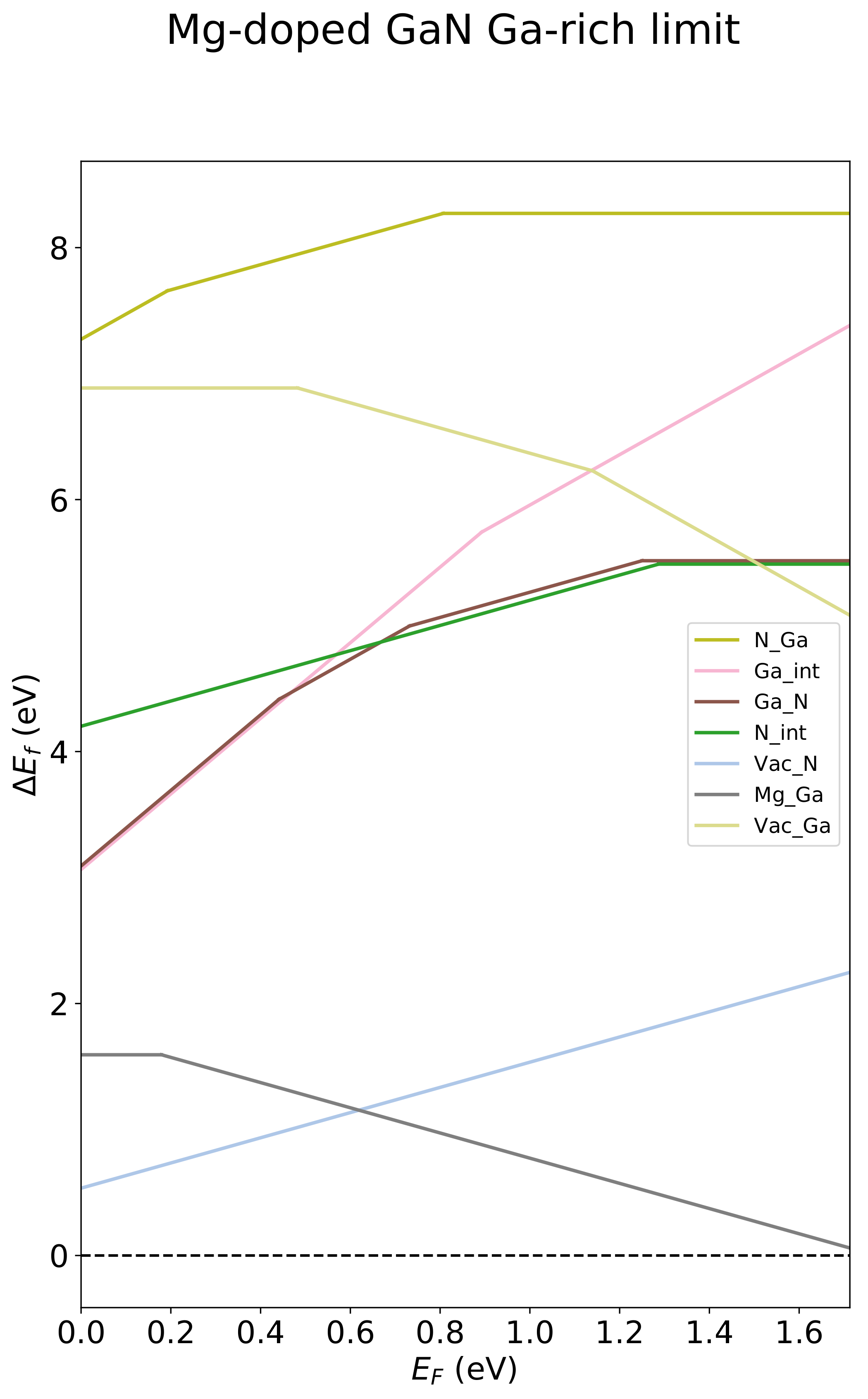
We can also plot a diagram showing the transition levels within the band gap:
defective_system.diagram.plot(save_flag=True,
                              title='Mg-doped GaN Ga-rich limit',
                              legend=True,
                              x_label=r'$E_F$ (eV)',
                              save_title='diagram_defsys')
Saves the file diagram_defsys.pdf:
Step 4. Calculate defect concentrations
Once defect formation energies have been calculated, it is also possible to calculate equilibrium defect concentrations in the dilute limit.
Spinney calculated defect concentrations through the EquilibriumConcentrations. An instance thereof is available in the DefectiveSystem instance.
To calculate the concentrations, we need to feed some more data to the DefectiveSystem instance. For more details about these quantities see Equilibrium defect concentrations in the dilute limit.
from spinney.io.vasp import extract_dos
import numpy as np

# get the density of states of the pristine system
dos = extract_dos('vasprun.xml')[0]

# site concentrations for point defects
volume = ase_pristine.get_volume()/ase_pristine.get_number_of_atoms()
volume *= 4
factor = 1e-8**3 * volume
factor = 1/factor
site_conc = {'Ga_N':4, 'N_Ga':4, 'Vac_N':4, 'Vac_Ga':4,
             'Ga_int':6, 'N_int':6, 'Mg_Ga':4,
             'electron':36 , 'hole':36}
site_conc = {key:value*factor for key, value in site_conc.items()}

defective_system.dos = dos
defective_system.site_concentrations = site_conc
# calculate defect concentrations on a range of temperature
defective_system.temperature_range = np.linspace(250, 1000, 100)

concentrations = defective_system.concentrations
We can now access equilibrium properties of interest, such as equilibrium carrier concentrations:
import matplotlib.pyplot as plt

carriers = concentrations.equilibrium_carrier_concentrations

# the sign is positive, except for very low temperatures:
# holes are the main carriers
T_plot = 1000/defective_system.temperature_range
plt.plot(T_plot, np.abs(carriers), linewidth=3)
plt.yticks([1e-10, 1, 1e10, 1e20])
plt.xlim(1, 4)
plt.yscale('log')
plt.title('Carrier concentrations')
plt.xlabel('1000/T (1/K)')
plt.ylabel(r'c (cm$^{-3}$)')
plt.tight_layout()
plt.show()

As the entry of carriers are always positive except for low temperatures, holes are the main charge carriers
in the system, meaning that the doping with Mg is effective at high temperatures, while holes are fast compensated
by intrinsic defects for lower temperatures.